Overview: The Future of AI-Generated Imagery

Key Highlights

Pixel MeanFlow (pMF) represents a groundbreaking image generation model designed for one-step generation. The core innovation of pMF lies in its ability to efficiently perform one-step generation within a latent-free, pixel-level modeling framework.

pMF operates directly in the raw pixel space, thus eliminating the need for pre-trained latent encoders (such as VQ-GAN or VAE). Despite this, it achieves generation quality comparable to that of state-of-the-art multi-step latent space diffusion models.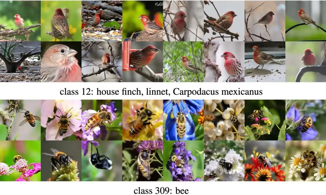

Problems Addressed

Modern generative models often face trade-offs across two fundamental dimensions:

• Sampling Efficiency: Multi-step sampling can produce high-quality results but suffers from slow inference speeds.
• Space Selection:
  • Latent Space: Reduces dimensionality through compression but introduces complex encoder/decoder architectures and sacrifices direct pixel-level control.
  • Pixel Space: Offers an intuitive "what you see is what you get" approach but poses significant challenges for modeling high-dimensional data.

Combining 'one-step generation' with 'pixel-space modeling' presents an extremely challenging task. A single neural network must simultaneously handle complex trajectory modeling and image compression/abstraction (manifold learning). Existing methods struggle to effectively balance both aspects.

Proposed Solution

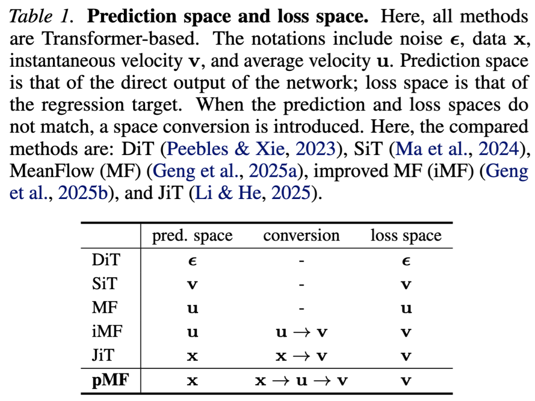
The core idea of pMF is to decouple the network's prediction target from the computation space of the loss function:

• Prediction Target: The network directly predicts the denoised 'clean' image (i.e., -prediction). Based on the manifold assumption, clean images lie on a low-dimensional manifold, making them easier for neural networks to fit.
• Loss Space: The loss function is defined in velocity space, following the MeanFlow formulation. It learns the average velocity field by minimizing instantaneous velocity errors.
• Conversion Mechanism: A simple conversion formula is introduced to establish a connection between the image manifold and the average velocity field. This enables the model to leverage the manifold structure of pixel space while performing effective trajectory matching in velocity space.

Applied Technologies

• Pixel-space Prediction: Directly parameterizes the denoised image in pixel space, leveraging the low-dimensional manifold assumption to reduce learning difficulty and avoid the challenges of directly predicting high-frequency noise or velocity fields.
• MeanFlow Formulation: Utilizes the Improved MeanFlow (iMF) framework to learn the average velocity field through losses in instantaneous velocity space.
• Flow Matching: Establishes a probabilistic flow from noise distribution to data distribution based on flow matching theory.
• Perceptual Loss: As the model directly outputs pixels, it naturally lends itself to the incorporation of perceptual losses (LPIPS and ConvNeXt features) to further enhance the visual quality of generated images, compensating for the limitations of pixel-level MSE loss.

Achieved Results

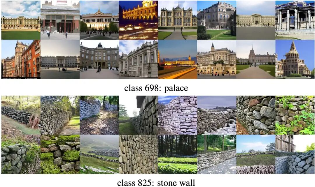
pMF demonstrates strong performance on the ImageNet dataset, proving the feasibility of one-step latent-free generation:

• ImageNet 256×256: Achieves an FID score of 2.22, surpassing many multi-step latent space models.
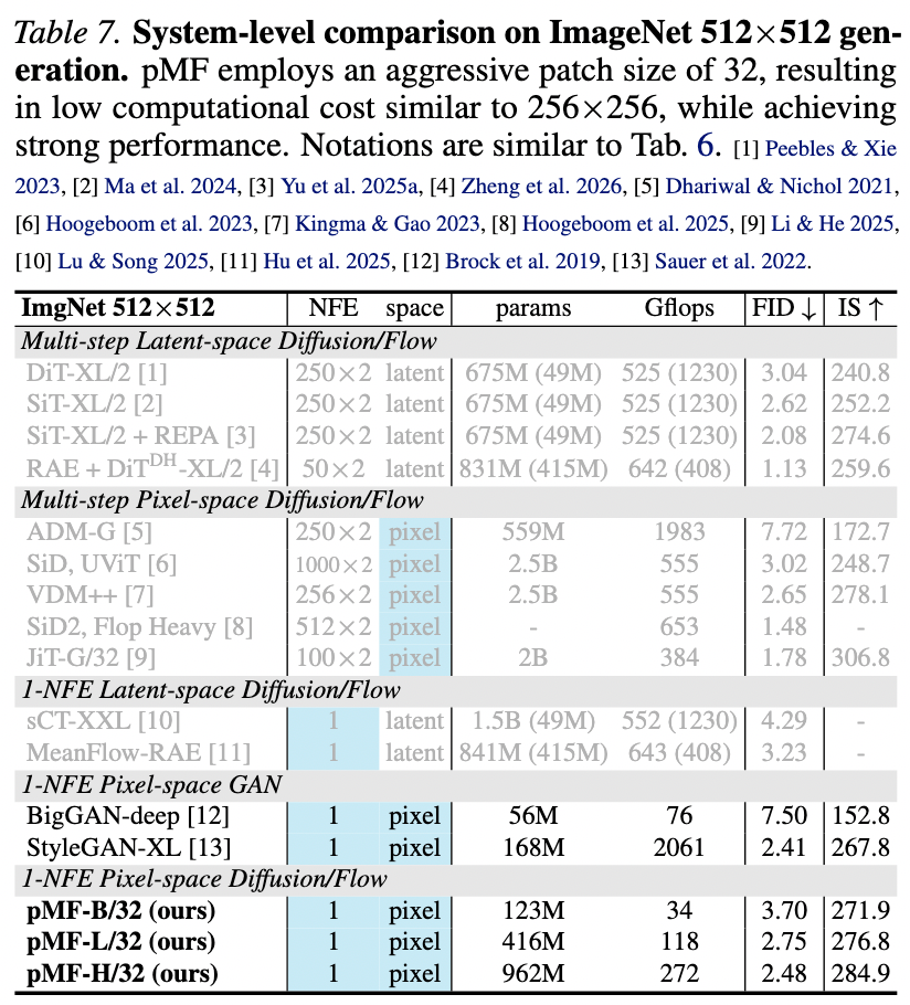
• ImageNet 512×512: Achieves an FID score of 2.48.

These results indicate that one-step pixel-level generation models have become highly competitive while eliminating the need for additional decoder overhead (which accounts for significant computational costs in latent space models).

Background

The development of pMF in this work builds upon Flow Matching, MeanFlow, and JiT.

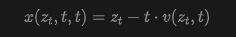
• Flow Matching: Flow Matching (FM) learns a velocity field that maps a prior distribution to a data distribution. This work considers a standard linear interpolation schedule: 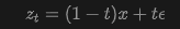where data , noise (e.g., Gaussian distribution), and time . At , we have: . This interpolation generates a conditional velocity : FM optimizes the network , parameterized by , by minimizing the loss function in -space (i.e., "-loss"): 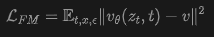Previous research (Lipman et al., 2023) has shown that the latent target of is the marginal velocity . During inference, samples are generated from to by solving the ordinary differential equation (ODE): , where . This can be achieved using numerical solvers such as Euler or Heun-based methods.
• Flow Matching with x-prediction: The quantity in Equation (2) represents a noisy image. To facilitate the use of Transformers operating on pixels, JiT chooses to parameterize the data via a neural network and converts it into a velocity using the following approach: 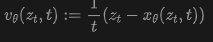where is the direct output of a Vision Transformer (ViT). This formulation is referred to as -prediction, while the -loss from Equation (2) is used during training. Table 1 outlines this relationship.
• Mean Flows: The MeanFlow (MF) framework learns an average velocity field for few-step/one-step generation. By treating FM's as instantaneous velocity, MF defines the average velocity as: where and represent two time steps: . This definition leads to the MeanFlow identity: This identity provides a method for defining the prediction function through the network : 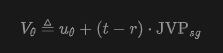Here, the uppercase corresponds to the left-hand side of Equation (6), while on the right-hand side, JVP denotes the Jacobian-vector product used to compute , and 'sg' indicates stop-gradient. This work follows the JVP computation and implementation of iMF, which is not the focus here. According to the definition in Equation (7), iMF minimizes the -loss, i.e., , similar to Equation (3). This formulation can be viewed as -prediction with -loss (see Table 1).

Pixel MeanFlow

To achieve one-step, latent-free generation, this work introduces Pixel MeanFlow (pMF). The core design of pMF establishes connections among different fields of , , and . This work aims for the network to directly output like JiT, while performing one-step modeling in and spaces like MeanFlow.

Denoised Image Field

As previously mentioned, both iMF and JiT can be regarded as minimizing losses in instantaneous velocity space (-loss), with the difference being that iMF performs average velocity prediction (-prediction), while JiT performs raw data prediction (-prediction). Based on this observation, this work establishes a mapping relationship between the average velocity and a generalized form of .

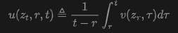
Consider the average velocity field defined in Equation (5): This field represents an underlying true quantity determined by the data distribution , prior distribution , and time scheduling, independent of specific network parameters . From this, we derive an induced field, defined as follows: As detailed below, this field plays a role similar to that of 'denoised images.' It is important to note that the defined in this work differs from the mentioned in previous literature, as it is a binary variable indexed by two timestamps : For a given observation , our is a two-dimensional field varying with , rather than a one-dimensional trajectory indexed solely by .

Generalized Manifold Assumption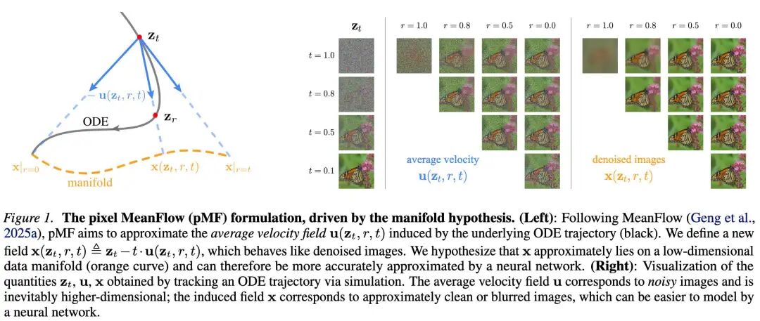

Figure 1 visualizes the and fields by simulating an ODE trajectory obtained from a pre-trained FM model. As shown, consists of noisy images because, as a velocity field, contains both noise and data components. In contrast, the field exhibits the appearance of denoised images: they are nearly clean images or blurry images resulting from over-denoising. Next, we discuss how the manifold assumption generalizes to this quantity .

Note that the time step in MF satisfies: . We first demonstrate that the boundary cases at and approximately satisfy the manifold assumption; then, we discuss the case of .

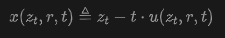
• Boundary Case I: . When , the average velocity degenerates into instantaneous velocity, i.e., . In this case, Equation (8) becomes: This is essentially the -prediction target used in JiT. Intuitively, this represents the denoised image that JiT aims to predict. If the noise level is high, this denoised image may appear blurry. As widely observed in classical image denoising research, it can be assumed that these denoised images approximately lie on a low-dimensional (or lower-dimensional) manifold.
• Boundary Case II: . The definition of in Equation (5) yields: . Substituting this into Equation (8) gives: 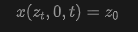which represents the endpoint of the ODE trajectory. For a true ODE trajectory, , meaning it should follow the image distribution. Therefore, we can assume that approximately lies on the image manifold.
• General Case: . Unlike boundary cases, the quantity does not guarantee correspondence to (potentially blurry) image samples from the data manifold. However, empirically, our simulations (Figure 1, right) indicate that resembles denoised images. This contrasts sharply with the velocity space quantity ( in Figure 1), which exhibits significantly more noise. This comparison suggests that modeling via a neural network may be easier than modeling the noisier . Experiments show that for pixel space models, -prediction performs effectively, while -prediction severely degrades.

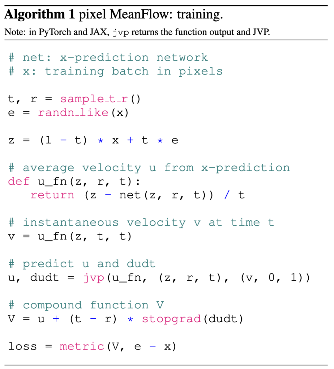
Algorithm

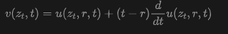
The induced field in Equation (8) provides a reparameterization of the MeanFlow network. Specifically, we let the network directly output and compute the corresponding velocity field via Equation (8): 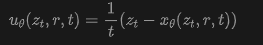Here, it represents the direct output of the network, following JiT. This formula is a natural extension of Equation (4).

This paper incorporates the from (11) into the iMF formula, specifically using Equation (7) with a -loss. Specifically, the optimization objective of this paper is: 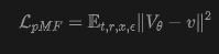where .

Conceptually, this is a -loss with -prediction, where is transformed into the space through the relationship of to regress . Table 1 summarizes this relationship. The corresponding pseudocode is in Alg. 1.

Pixel Averaging Flow with Perceptual Loss

The network directly maps noisy input to a denoised image. This enables a 'what you see is what you get' behavior during training. Therefore, in addition to the loss, this paper can further incorporate a perceptual loss. Potential-based methods benefit from perceptual loss during tokenizer reconstruction training, while pixel-based methods have not yet been able to leverage this advantage.

Formally, since is the denoised image in pixels, this paper directly applies a perceptual loss (e.g., LPIPS) to it. The overall training objective of this paper is , where denotes the perceptual loss between and the real clean image , and is a weight hyperparameter. In practice, the perceptual loss is only applied when the added noise is below a certain threshold (i.e., ) to prevent the denoised image from being too blurry. This paper investigates both the standard LPIPS loss based on a VGG classifier and a variant based on ConvNeXt-V2.

Relation to Previous Work

The pMF in this paper is closely related to several previous few-step/one-step methods, discussed as follows.

• Consistency Models (CM): Learn a mapping from noisy samples directly to generated images. In this paper's notation, this corresponds to a fixed endpoint . Additionally, CM typically employs a pre-conditioner in the form of . Unless is zero,

  Figure 2 illustrates that -prediction performs reasonably well, whereas -prediction deteriorates rapidly as increases. This study observes that this performance disparity is mirrored in the training losses: -prediction yields a lower training loss compared to its -prediction counterpart. This implies that predicting is more manageable for a network with limited capacity.

  Experiments on ImageNet

  This study carries out ablation experiments on ImageNet at a default resolution of 256×256. FID scores are reported based on 50,000 generated samples. All models generate raw pixel images through a single function evaluation (1-NFE).

  The Network's Prediction Target

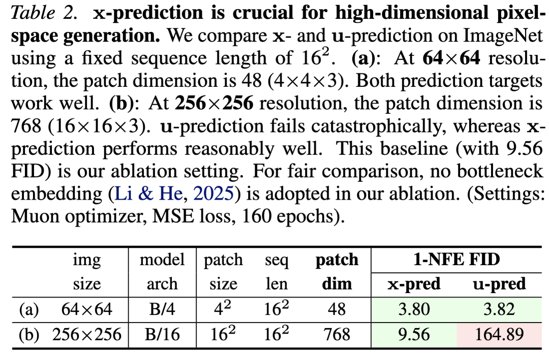
  The methodology employed in this study is grounded in the manifold hypothesis, which posits that resides on a low-dimensional manifold and is thus easier to predict. This hypothesis is validated in Table 2.

  64×64 Resolution: The patch dimension is 48 (). This dimension is notably lower than the network's capacity. The results indicate that pMF performs effectively under both -prediction and -prediction.

  256×256 Resolution: The patch dimension is 768 (). This leads to a high-dimensional observation space, posing a greater challenge for neural networks to model. In this scenario, only -prediction performs satisfactorily (FID 9.56), suggesting that lies on a lower-dimensional manifold and is hence more amenable to learning. Conversely, -prediction suffers a catastrophic failure (FID 164.89): as a noisy quantity, has full support in the high-dimensional space, complicating its modeling.

  Ablation Study

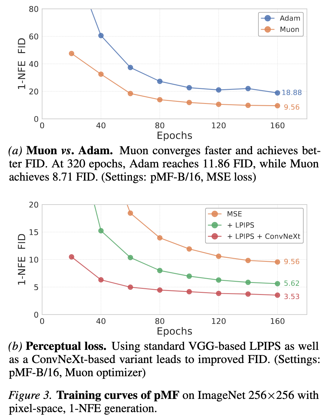
  Optimizer: This study identifies that the choice of optimizer significantly impacts pMF. In Figure 3a, the standard Adam optimizer is compared with the recently proposed Muon. Muon demonstrates faster convergence and a substantially improved FID (from 11.86 to 8.71). In a one-step generation setting, the advantage of faster convergence is further accentuated, as a superior network provides a more precise stopping gradient target.

  Perceptual Loss: In Figure 3b, this study further integrates a perceptual loss. Employing the standard VGG-based LPIPS enhances the FID from 9.56 to 5.62; combining it with the ConvNeXt-V2 variant further refines the FID to 3.53. Overall, incorporating the perceptual loss yields an improvement of approximately 6 FID points.

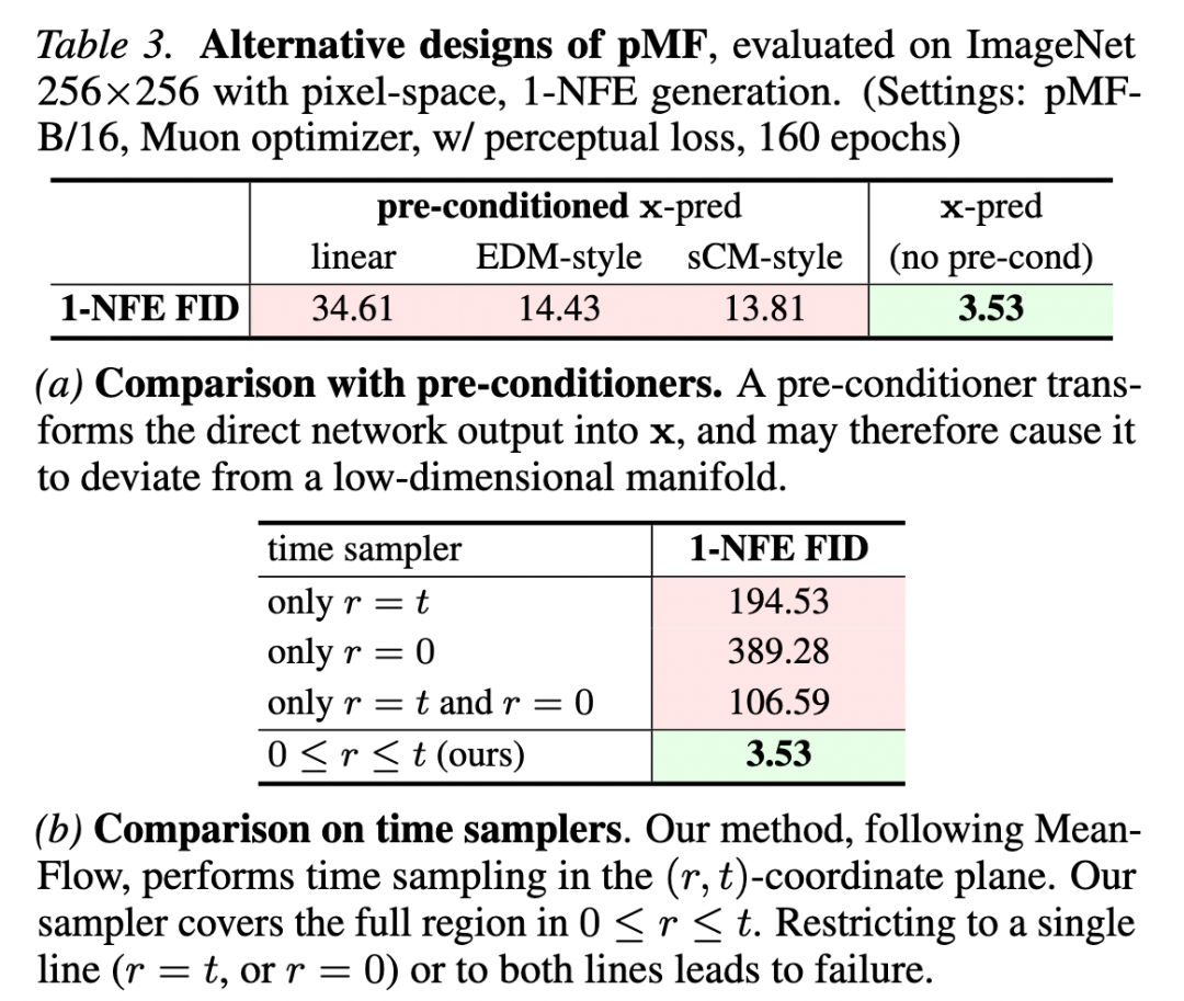
  Alternative: Pre-conditioner: This study compares three pre-conditioner variants: (i) linear; (ii) EDM style; (iii) sCM style. Table 3a reveals that while EDM and sCM styles outperform the naive linear variant, simple -prediction is more preferable and performs better in the extremely high-dimensional input regime considered in this study. This is because unless , the network prediction diverges from the space and may reside on a higher-dimensional manifold.

  Alternative: Time Sampler: This study explores alternative designs for restricting time sampling: only (i.e., Flow Matching), only (akin to CM), or a combination of both. Table 3b indicates that none of these restricted time samplers suffice to tackle the challenging scenarios considered in this study. This suggests that the MeanFlow method capitalizes on the relationship between points to learn the field, and restricting time sampling may disrupt this formulation.

  

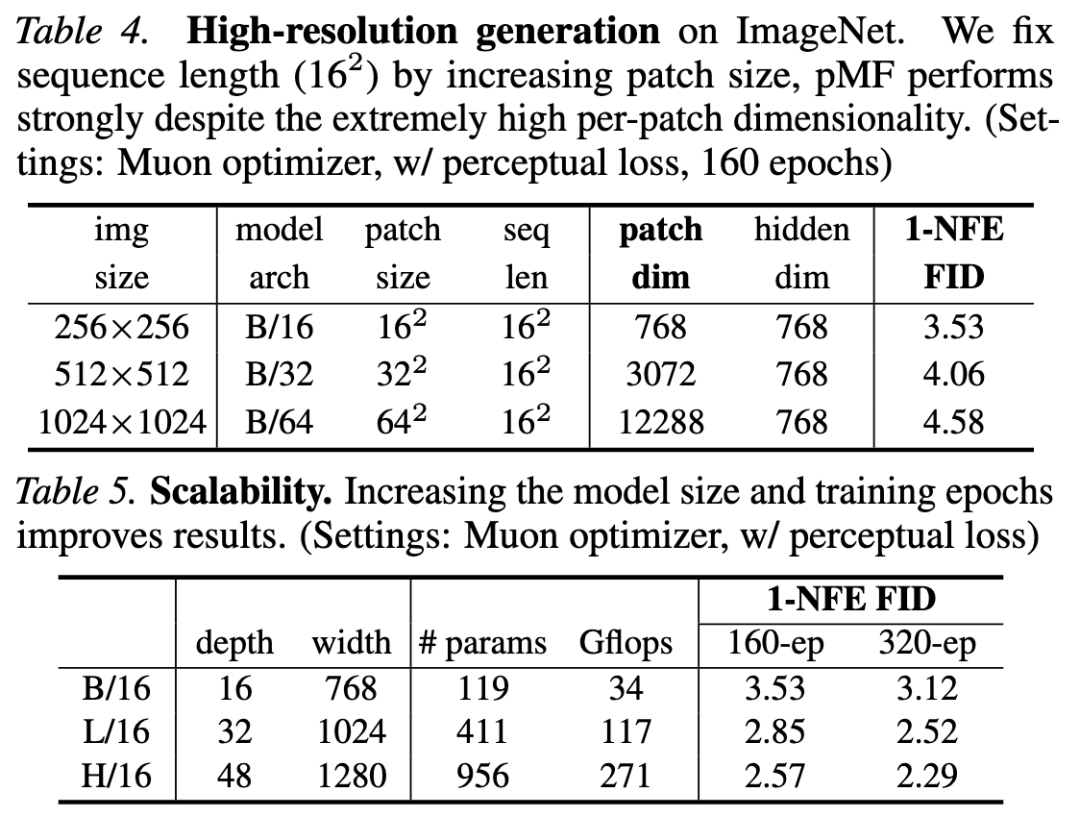
  High-Resolution Generation: In Table 4, this study investigates pMF at resolutions of 256, 512, and 1024. By increasing the patch size (e.g., ) to maintain a constant sequence length (), it results in an exceptionally large patch dimension (e.g., 12288). The results demonstrate that pMF can effectively manage this highly challenging scenario. Even though the observation space is high-dimensional, the model consistently predicts , whose latent dimension does not scale proportionally.

  Scalability: Table 5 indicates that augmenting both the model size and training duration enhances the results.

  

  System-Level Comparison

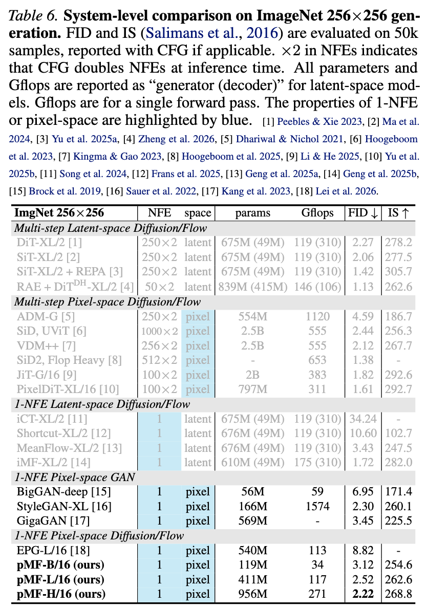
  ImageNet 256×256: Table 6 reveals that this study's method achieves an FID of 2.22. To the best of this study's knowledge, the only method in this category (one-step, latent-free diffusion/flow) is the recently proposed EPG, which has an FID of 8.82. Compared to leading GANs, pMF attains a comparable FID but with significantly reduced computational demands (e.g., StyleGAN-XL necessitates 5.8 times more computation than pMF-H/16).

  

  ImageNet 512×512: Table 7 shows that pMF achieves an FID of 2.48 at 512×512. Notably, its computational cost (in terms of parameter count and Gflops) is comparable to its 256×256 counterpart. The only additional overhead arises from the patch embedding and prediction layers.

  

  Conclusion

  Fundamentally, an image generation model is a mapping from noise to image pixels. Owing to the inherent challenges of generative modeling, this problem is frequently decomposed into more manageable subproblems involving multiple steps and stages. While effective, these designs deviate from the end-to-end ethos of deep learning.

  This study's research on pMF demonstrates that neural networks are highly expressive mappings and, when appropriately designed, can learn complex end-to-end mappings, such as directly from noise to pixels. Beyond its practical potential, this study hopes that this work will inspire future exploration of direct, end-to-end generative modeling.

  References

  [1] One-step Latent-free Image Generation with Pixel Mean Flows